INTRODUCTORY TUTORIAL FOR IPP'S WEBSITE

1) Are You Curious About Causes?

We invite you to join us in a fascinating adventure. We are going to plunge into the hidden depths of physics, to see if we can discover what makes Nature tick. We realize that you will be wary, and will want answers to a number of questions, before we start:

Q: Where will we be going?
A: To a place, where we can see the fundamental building blocks of the universe.

Q: Where is this place located?
A: Anywhere in the universe that our imaginations can go.

Q: How will we know when we get there?
A: We will see myriads of exceedingly tiny spheres, all jammed into contact with each other.

Q: How small will these spheres be?
A: About 0.2 fermi in diameter (2x10 ^–14 cm), which is about 1/10 the (currently accepted) size of a hydrogen nucleus.

Q: How many of these spheres will we expect to find?
A: Countless! Somewhat more than 10 ⁴¹ per cubic centimeter; very likely more than 10 ¹²² in the observable universe!

Q: What shall we call these tiny spheres?
A: Elemental Charge Entities, or, more commonly, +ECEs & -ECEs.

Q: So these spheres possess charge?
A: Yes! They have a charge of ±1/2e, or half a positron's, or electron's charge.

Q: What role do ECEs perform in physics?
A: They are the root cause of everything! They are the only material objects that exist in the universe, and their interactions produce all the observed (and inferred) phenomena of physics!

Q: You expect me to believe that?
A: Not right away! But, if you are willing to look carefully at all the animated, three-dimensional drawings on this website, click on, and read all the explanatory notes, and study with diligence the website introduction, and the enclosed textbook, Infinite Particle Physics, we will bet you even money that you will come back from your journey convinced!

2) The Current View Of Space

Main line physicists currently view space as emptiness infused with infinitesimal points of matter. They assert that these points position themselves, and induce movement relative to each other, through a process of emitting and catching a variety of massless ghost-like force particles. These ghost particles are also considered to be infinitesimal points.

3) IPP's Concept Of Space

IPP views space as an agglomeration of elemental charge entities (hereafter, ECEs). ECEs are postulated to be tiny rigid spheres of ±1/2e charge that form a dense, but deformable, structure extending to the boundaries of the observable universe. The new theory postulates that these tiny ion-like spheres are created in too much abundance to form a perfect simple cubic lattice, but, instead, tend to form a slightly "squashed" (rhombic) polycrystalline cubic lattice laced with a multitude of defects and lattice-density oscillations that create infinitely extending dynamic distortion patterns. These infinite dynamic distortion patterns are IPP's concept of matter & energy.

4) Training Your Imagination

Infinite Particle Physics is about the mechanisms of physical phenomena. Understanding these mechanisms requires that you first learn how to visualize, in three-dimensions, the central regions of the infinite distortion patterns that IPP associates with photons, leptons, mesons, baryons, and nuclei. Then, you will need to learn how to perceive these objects, not as fixed shapes, but as dynamic patterns that modulate their shapes continuously between two limits in a cyclical manner. Next, you must learn how to imagine these changing shapes in their actual sizes. This requires mentally shrinking the cores of these imagined images to sub-fermi dimensions, while simultaneously expanding their boundaries to infinity! Finally, having acquired the ability to visualize the dynamic shapes of all the important types of phenomena, you should be able to understand how these various types of phenomena interact with each other (and with all other phenomena in the universe) to alter each other's dynamic shapes, and what the consequences are of these alterations.

5) Getting The Most Out Of IPP's Drawings

The purpose of an IPP drawing or schematic is to help you form a 3-D moving picture in your mind of some specific aspect of physics. In viewing these drawings, you must understand that they can portray only a static snapshot, or an animated sequence of changing snapshots, of a minute portion of a dynamic & infinitely extending lattice distortion pattern. Thus, there is not nearly enough information in any particular drawing to let you form the mental moving picture of infinite scale that IPP hopes to impart to you. You may need to look at dozens of drawings, and read the accompanying texts, before you can view a static drawing, and see it as an inverse-square decremented, incessantly oscillating lattice disturbance interpenetrating & interacting with the infinitude of similar structures in the cosmos.

My assistant, Jason Smith, has made all the drawings on the website. Many just duplicate, in modern clothes, drawings that I had made over twenty years ago. (For examples of these earlier drawings see the online textbook.) But these modern clothes make a world of difference! They have helped both of us learn new concepts about infinite particles, especially about their dynamics. When we try to animate our mental pictures of particle dynamics, these drawings with full-scale ECEs make clear the constraint imposed by IPP's notion of "cosmic excess of ECEs", which requires that ECEs maintain "touching" relationships (tangency) throughout their dynamic excursions.

For example, when we try to show the excursions of ECEs through a cycle of a point-centered lattice density oscillation, any improperly programmed ECE pathways of the collapsing & uncollapsing lattice result in visible merging of ECEs in some parts of the cycle. Here is clear indication that we have used faulty programming logic! Usually this merging of ECEs has resulted from attempting to use conventional equations to program the ECE motions. When we show you the solution to these ECE intersections in the drawings soon to follow, you will understand why only geometric reasoning can discover the appropriate logic. You will also see that our geometric logic yields insights into the polarization of light that are not revealed by the current approach.

6) Symbols Used To Represent ECEs In Our Drawings

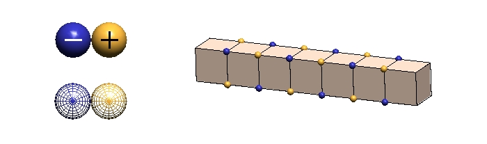
Minus ECEs and plus ECEs will normally be portrayed as blue and gold spheres, of varying size. Occasionally, we will represent some of the ECEs as semi-transparent, wire-framed blue & gold spheres. These will be used to call attention to signficant features of a drawing, often being "blinked" for this purpose. Sometimes we want to de-emphasize parts of a drawing. We show the ECEs of these parts as small spheres at nodes in a cubic lattice. Examples of theses drawing conventions are shown below:

7) IPP's Space \ Energy Structures

In the INTRODUCTION, I explained that the central mechanics of an IPP particle is a permanently-bound combination of a lattice defect with a point-centered ellipsoidal lattice-density oscillation. Thus, in order to understand the nature of IPP's particles, we must learn how to form moving pictures in our minds of the dynamic distortion patterns that each of these phenomena produces, and then we must learn how to merge them together into a composite image. Let's begin with the distortion patterns produced by lattice-density oscillations. We will investigate those produced by lattice defects later in this article.

The word, oscillation, implies continuous back and forth movement of something between two limits, so let us think about what these limits might be for a point-centered spherical lattice-density (LD) oscillation (the non-drifting form of an ellipsoidal LD oscillation) in the packing density of particles comprising a space lattice. Here are some things we need to consider in determining these limits:

• Each point-centered dynamic distortion pattern (whether particle or energy, whether stationary or moving) owes its existence to having captured a discrete amount of cosmic shrinkage.



• This discrete amount of captured shrinkage is not concentrated at the pattern's center, but, rather, is distributed in equal radial increments to infinity (except for the central region, as noted later).



• If a LD oscillation is stable (i.e., possessing an unvarying amount of captured shrinkage), any variations in the packing-density of ECEs in one radial zone (i.e., in a spherical shell) must be offset by equal and opposite variations in packing-density in an adjacent zone, in order to keep the total shrinkage constant.



• Hence, we should visualize a spherical LD oscillation as in-and out movements of spherical shells of varying ECE packing densities whose amplitudes of variation scale as the inverse-square of their radial distances from the pattern center. For those interested in why LD oscillations occur in space, please see my discussion in Chapter 1 of the online textbook.

Now, let us see why the amplitudes of ECE packing-density variations of an LD oscillator must deviate from the inverse-square of radius in its central region. Here are the arguments:

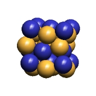
Although, mathematically, we would expect an LD oscillator's center to have infinite amplitude of density variations, we can readily perceive that there will be a density maximum in IPP's postulated space of always "touching" spherical ECEs. This limit will be reached when ECEs have rotated around each other until the void spaces between them have reached a minimum, as I show in the center figure, below. IPP calls this ECE maximum-density configuration, "saturation".

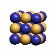
The minimum of an LD oscillator central variation of ECE density would seem to be the limit reached when the lattice takes the form of the undistorted simple cubic lattice of "empty" space, as in the left picture below. Although this "empty" space state seems obviously the least "saturated" lattice condition, it is clearly not a stopping point in an oscillation since all the ECEs returning from the saturated state can continue their motion until they reach another state of "saturation" with the reverse character of the first "saturated" state. (This back-and-forth movement is the subject of Section 8.)

Simple Cubic Lattice (Empty Space)	Saturated Space (Mass-Energy Center)	Body-Centered Cubic Lattice (Black Hole)

8) Cardinal Asymmetry Develops In Saturated Space Oscillations

You will notice in the animated drawings of a lattice-density oscillation, below, that the local ECEs move in a pattern that causes the lattice to change from the simple cubic lattice structure of "empty" space to a "jammed-together" form IPP calls "saturated space", then back again through simple cubic space to saturated space of an opposite character. If you follow the motion of a single ECE, you will see that it moves back and forth from its "empty space" location in a lattice cube-diagonal direction, and therefore is moving most rapidly as it goes through "empty space", where there is the most room for it to move.

Although the details are too complex to enter into now, I think you will see that there is sufficient complexity of movement of adjacent ECEs to imagine that opposite-polarity ECEs could exchange their respective locations if their movements were complicated by the presence of lattice defects that introduced charge irregularities into the central structure, particularly if the center of the lattice-density oscillation were continually shifting because of its ellipticity.

Lattice Density Oscillation Center (XY Plane)	Lattice Density Oscillation Center (XYZ Planes)

Notice, above right, that, at saturation, the plus and minus ECEs of the x-z planes form displaced planes in the y-direction, but that opposite-polarities ECEs nest together in the x-y planes & in the y-z planes. Since IPP postulates that photons are ellipsoidal lattice-density oscillations that lack a central defect, I have suggested that this asymmetry may explain why photons manifest the phenomenon of polarization. An interesting thing to notice about this explanation of polarization is that its absolute orientation in space must shift, as the central saturation zone transits from crystal to crystal in polycrystalline space. Perhaps this shift of its polarized direction as a photon moves through space may help explain some of the baffling effects that quantum physicists have noticed.

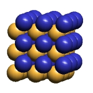
Notice also that the charge layering in the y-direction of the saturated pattern begins to approach the precise layering of the body-centered cubic form of section 7). This lends credence to IPP's suggestion that the body-centered cubic lattice is the product of even further ECE packing-density increases (lattice compression), and thus is plausibly the structure of a black hole.

Now let us examine these saturated lattice structures in more detail:

9) Determining ECE Motions That Lead From Simple Cubic Lattice To Saturation

When we seek to understand how the lattice collapses to maximum compaction (saturation), we find that IPP’s notion of always “touching” ECEs places some rather unusual constraints on individual ECE movements. It seems clear enough that the least encumbered direction of motion of any individual ECE would be along a lattice cube diagonal, but, of course, only two of the lattice cube’s eight ECEs could move inwardly, and these would have unobstructed movement only if the other six ECEs moved outwardly, toward the centers of adjacent lattice cubes. And these six ECE movements would require the coordinated movements of the other ECEs in these adjacent cubes, etc. These complex patterns can be worked out by using the following procedure:

1. Assume a simple cubic lattice of “touching” ECEs, where the center of each ECE has integer coordinates x, y, z relative to the center of a central ECE.



2. For each point, determine whether the x, y, z coordinates are odd (O), or even (E). This can be achieved by using modulus (2) operation on each axial coordinate.



3. Use the logic table, below, to determine which direction each ECE needs to move to produce lattice compaction. Saturation will be produced when the appropriate signs are prefixed to
   
   for each ECE of the pattern. Reversing all the signs yields the reverse saturation pattern.



4. Notice that the lattice constant, ü, must shrink as the degree of compaction increases, reaching a value of 0.917 at saturation.

Logic Table

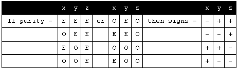
You will notice that the logic requires one of the three coordinates (in this case, the y) to exhibit an unchanging parity sequence, while the other two coordinates have inverted sequences in the two options. This is the explanation for the asymmetry of the saturation pattern, where we see polarized faces in the fixed sequence direction, and neutralized faces in the other two coordinate directions. This asymmetry of pattern is persuasive as an explanation for the polarization of light, since the inverse-square diminished oscillatory pattern must follow the same logic.

10) How Central Saturation Affects The Radial Distribution Of Mass-Energy

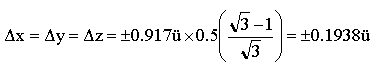
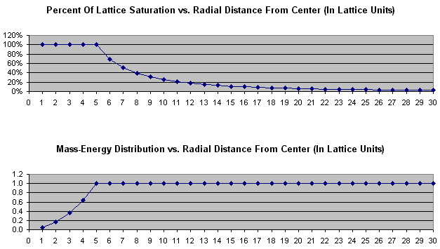
Our deduction that the oscillator's shrinkage (mass-energy, E) is distributed in radial equal increments to infinity cannot be valid in an oscillator's central saturated zone. Instead we see that DE / D r must increase outwardly from the saturation zone center to its perimeter, because saturation implies a constant amount of shrinkage per unit volume, and the saturation volume varies as the square of the radius increment. The two curves below suggest how we should alter our thinking about the radial distribution of mass-energy when an oscillator's zone of saturation has a radius of 5ü.

11) The Radius Of Saturation Zone vs. Oscillator Mass-Energy (E)

The concept of a central saturation zone solves the problem of infinite central amplitude that plagues a simple mathematical formulation of a point-centered spherical lattice-density oscillation. But this solution still leaves us with the problem of correlating the size of the saturation zone with a particular amount of oscillator mass-energy (E). We can infer that its radius increases as E^1/3, but how do we find the mass-energy value that correlates with a radius of 1ü? Let's speculate about this:

We can infer that a non-drifting lattice void (IPP's muon neutrino) requires central ECE motions of at least 1ü/, in order for it to hover in the space lattice. Thus, we must presume that it requires a central saturation zone of at least 1ü radius. In Chapter Eight of the online book (see pg. 8-9), in my analysis of redshift in a static universe, I show why we should infer that the mass-energies of two separated opposite-polarity voids should differ from the mass-energy of a void pair (IPP's electron neutrino) by only about one milli-eV (the mass-energy released by the cancellation of the charge fields of the two joining voids). If we tentatively accept LBL's value for the mass-energy of an electron neutrino, and use a radius value of 1ü for it, we can find the saturation zone radii (SZR) for the following particles:

12) Picturing The Simple Defects That Occur In IPP's Space

Leptons, from IPP's perspective, are dynamic distortion patterns that are centered upon single lattice defects (or an opposite-charge pair of single lattice defects), each of which occurs in two polarities: ± void defects, ±± replacement defects, & ± excess defects. And, like hadron distortion patterns, lepton dynamic distortion patterns result from a combination of a defect and a point-centered ellipsoidal lattice-density oscillation bound together through mutual entanglement*.

* Entanglement results from mutual feedback, whereby the defect's charge field causes the oscillator's center to retreat from it, while, simultaneously, the circling movement of the central ECEs (induced by the oscillation) causes the defect to change its location to the opposite side of the oscillator's center, where its charge field now repels the oscillator's center in the reverse direction. Entanglement occurs during the central rarefaction phase of the bound LD oscillator, when its central ECEs are moving most rapidly around each other (i.e., when the central ECEs are midway between one saturation orientation and the other). All these feedback processes reverse, of course, during the next central rarefaction phase, causing the defect to circle back to its original location, because all the central ECEs are moving in opposite directions. The circling movements of the central ECEs, which produce the defect's circling translocation, are the basis of IPP's explanation of lepton spin.

Let's look at the distortion patterns of each of these defect types. We shall begin with the lattice voids.

Why IPP Identifies Voids As (Charged) Muon Neutrinos:

Particle physicists currently assume that muon neutrinos and muon antineutrinos are neutral particles, because:

1. These particles do not reveal themselves (don't leave trails) in any particle detectors.



2. They assume that muons have the same charge as electrons & positrons, and, hence, charge could not be conserved in the decay, ± pion ® ± muon & muon neutrino, unless the latter particle had zero charge.

IPP asserts that these experimental findings are also consistent with assigning a charge of ± 1/2e to both muons and muon neutrinos, because:

1. Half-charge particles of the presumed very low mass-energy of lattice voids would be incapable of deflecting electrons sufficient to produce ionization in particle detectors.



2. Decay of a ± pion (IPP's ± defect-pair) would conserve charge in producing IPP's half-charge excess defect & half-charge void defect.

There are other persuasive arguments in favor of IPP's choice, which I explore on page 1-28 of the online book. Here are two of the most convincing of these:

1. If a muon is a half-charge particle, it becomes clear (and solves a half-century of bafflement) why it cannot decay electron/gamma, as experiment forces us to conclude.



2. The half-charge muon neutrino provides a simple explanation for the so-called "neutral-current effect" in which a proton is deflected by the (presumed) close encounter with a relativistic muon neutrino. (This deflection is currently explained by the presumed emission of a Z-particle by the muon neutrino, which is presumed caught by the proton, or vice versa).

How A Void Moves Through The Space Lattice

The movement of a very low mass-energy particle like a void raises an interesting puzzle. If the frequency of its hovering oscillation is set by E = hf, we must try to understand how it can attain high velocity with very little increment of momentum, i.e., how does it translate through many lattice-units of distance per cycle of its hovering oscillation. We illustrate, below, the basic concept, whereby a void can change its lattice location by eight face-diagonal lattice units through the movement of a face-diagonal column of eight like-charge ECEs. This is, of course, just the barest start of an explanation. There are many ancillary complications, which only further study will resolve.

IPP's Concept of An Electron Neutrino (A Void-Pair)

IPP's proposed structure for an electron neutrino is an electrostatically bound pair of opposite-charge voids, which translate back and forth past each other unceasingly under the influence of their synchronized hovering oscillators, as shown in the drawing below. Although each void generates an electrostatic field when they are separated, the two fields are essentially completely cancelled by their back and forth motions. Therefore, remote from this translational dynamic, the void-pair exhibits zero charge, and thus will interact with surrounding matter as a neutral particle. IPP's notion of an electron neutrino is persuasive, because:

1. It supports the experimental finding that electron neutrinos differ from muon neutrinos in their observed reactions with nucleons, wherein the relativistic electron neutrino interactions always yield an electron among the decay residues, while relativistic muon neutrinos always yield a muon among the decay residues.



2. It explains why electron neutrinos are less massive than muon neutrinos, as experimentalists infer, because the joining of the two voids cancels the mass-energy embodied in each void's electrostatic field.

IPP's Concept Of An Electron/Positron (±± Replacement Defect)

A replacement defect is a dynamic distortion pattern resulting from the removal of an ECE of either polarity from any location in the lattice, and replacing it with an ECE of opposite polarity. Since both the removal and the replacement results in a half-charge imbalance of the same polarity, a replacement defect's distortion pattern generates an electrostatic charge effect of ±e. IPP suggests that one can visualize this electrostatic field as an asymmetry in the dipole rotations of adjacent plus & minus ECEs as they oscillate back and forth (in infinite inverse-square-decremented fashion) in response to the defect's bound hovering oscillator. Electrostatic fields are only one component of a replacement defect's dynamic distortion pattern; the other components are defect hovering (spin), shrinkage (gravity), and oscillator ellipticity (drift velocity).

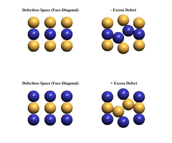
It is very challenging to attempt to visualize any defect's distortion pattern in its full dynamic complexity, so we must start simple! Below, left, is the configuration of ECEs in "empty" space, while, on the right, is the configuration of ECEs we identify as a stop-action picture of our minus (or plus) replacement defect at its hovering oscillator's moment of minimum central "saturation" (i.e., when the oscillator's center takes on the structure of "empty" space). If we think back to our (Section 8) dynamic picture of an LD oscillator's "saturation" & "unsaturation", we recall that all these nine ECEs are presumed to be moving at their maximum oscillatory velocity, in diverse cube-diagonal directions, with built-in asymmetry in their pattern of movement. To this complex motion, we must now mentally add the effect produced by the out-of-place charge of the replacement ECE on all these diverse movements, if we are to perceive the replacement defect's dynamics. Obviously, much mental work needs to be done!

Replacement Defect (Electron/Positron)

Electron Translocation

Electron/Positron Pair Creation

Excess Defect (Muon)

IPP chooses ± excess defects as its concept for muons for three reasons:

1. We assume that leptons are distinguished from hadrons by being single defects, rather than defect-pair clusters, and the excess defect is the only single defect thus far unassigned (after choosing lattice voids for neutrinos, and replacement defects for electrons & positrons).



2. We perceive that forming an excess defect structure requires squeezing an additional ECE into some site in a neutral simple cubic lattice, and this action will create considerably more point-centered rhombic distortion than is created by either a void or a replacement defect, since these defects exhibit perfect spherical symmetry. Thus, in view of the fact that we equate rhombic distortion with lattice shrinkage, and lattice shrinkage with mass-energy, we see that much more mass-energy must be captured to form "excesses", than to form "voids" or "substitutions". Although we don't yet know how to quantify the various amounts of mass energy absorbed in forming these three lepton defect types, we do know the mass-energy value for the somewhat similar rhombic distortion produced by a paired c-void (136/2 MeV). This c-void mass-energy value is suggestively close to 105/2 MeV, which would be the muon's mass-energy determined from e/m measurements, if one were to assume that the muon has IPP's suggested charge value of ± 1/2e.



3. We are even pleased that IPP's excess defect has a charge of ± 1/2e (rather than QCD's ±e muon), because this explains why a muon is never observed to decay electron/gamma. Half-charge muons also justify IPP's choice of a ± 1/2e charge void for its muon neutrino, which choice, in turn, distinguishes it from IPP's electron neutrino (a neutral ± void-pair).

The Creation (Formation) Of Excess Defects

When excess defects are created from a zone of undedicated shrinkage*, they will always be produced in opposite-polarity pairs. The production scenario, during the oscillators' synchronized central rarefaction phase, will resemble that shown in the animated drawing immediately above for electron/positron creation, but the onset of the oscillators' saturation phase will be much more abrupt, due to the much higher oscillatory frequency associated with the much higher mass-energy required for excess defect creation. What we should imagine happening in this higher frequency environment is that the two chains of ECEs moving in opposite face-diagonal directions toward the adjacent oscillator centers will be squeezed together lengthwise. This action will tend to make these columns fold like an accordion, such that the two closest to the oscillator centers will orient in a lattice cube-diagonal direction, where maximum room exists to accommodate them.

* IPP's term, undedicated shrinkage, has a specific, but nebulous, meaning. It refers to the oscillatory lattice structures that we infer must exist between the moment that mass-energy is released by matter-antimatter annihilations or momentum cancellations, and its utilization in the production of subsequent physical phenomena. The undedicated shrinkage that I visualize for the above creation scenario is a lattice structure of two closely adjacent point-centered lattice-density oscillations, sharing equally in the released mass-energy, and forced to oscillate at the same frequency by virtue of their proximity.

The instantaneous central lattice patterns that are created in each of the two oscillator centers by lattice cube-diagonal accommodation are shown below. We show only the immediately surrounding ECEs in the respective face-diagonal planes in which these ECEs lie. We trust, by now, that you have developed sufficient visualization skills, so that you can visualize this static lattice pattern of ± excesses in 3-D. Obviously this is just the barest start. Visualizing the full dynamics of the drifting excess defect over the entire hovering cycle lies well into the future!

Excess Defect (Muon)

Tau Leptons

There is nothing in IPP theory to suggest that tau leptons exist. I have found a very acceptable defect-pair structure, a variant of (structurally) a D-type meson, that yields the precise tau mass, and plausibly decays into all the observed tau decay modes (Please see the hadron tutorial for discussion about the tau meson). There aren't any defects that I can think of that would correlate with a tau lepton or a tau neutrino, so I must contest the current belief of particle physicists that the tau exists. I am content to let future physicists prove me right, or wrong. I know which way I would bet!

Collapsed-Void Defect (IPP's Alternative To QCD's Quarks)

You will find the discussion about this defect in the hadron tutorial, accessible through the navigation bar to your left.

END OF TUTORIAL